Quadrotto - control

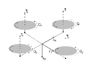
A quadrotor is composed by 4 electric motor-fixed step rotor modules fixed at the tip of 2 bars arranged as a cross. On center part of the vehicle there's a support for avionics. Vehicle is controlled inclining the model and thus the traction vector (in a first approximation normal to the rotors plane). Each rotor traction is controlled changing motor's rpm: in this way we can control trajectory and Euler angles. Figure below is a scheme with indicated blades rotation direction (same sign for rotor on the same bar) and aerodynamic couple (Q_i).

Mathematical model

On state space, motion equation can be written as:

$\begin{displaymath} \dot{x} = f_0(x)+F(x,u) \end{displaymath}$

(1)

where

$\begin{displaymath} x = [N E D u v w \phi \theta \psi p q r] \end{displaymath}$

(2)

is the state variables vector with (N,E,D) the coordinates of center of mass, (u,v,w) and (p,q,r) the components of, respectively, linear velocity and rates of turn, (φ,θ,ψ) the Euler angles, and

$\begin{displaymath} u = [{\omega}_{r_1} {\omega}_{r_2} {\omega}_{r_3} {\omega}_{r_4}] \end{displaymath}$

(3)

is the input variables vector where each element is the i-th rotor's rates of turn. Then

$\begin{displaymath} f_0(x)=[(R^{-1}\Omega_B)^T (-\Omega_B\times V_B)^T (L_{EB}V_B)^T\times (-I_B^{-1}[\Omega_B\times I_B\Omega_B]) ]^T \end{displaymath}$

(4)

where I_B is the inertia tensor, L_EB is the transformation matrix, other symbols have the known meaning and

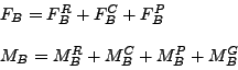
$\begin{displaymath} F = [ 0^T \frac{F_B^T}{m} 0^T (-I_B^{-1}M_B)^T]^T\in \Re^{12} \end{displaymath}$

(5)

is the generalized forces vector. Force F_B and moment M_B can be written as

$\begin{displaymath} \begin{array}{l} F_B = F_B^R + F_B^C + F_B^P\\ \\ M_B = M_B^R + M_B^C + M_B^P + M_B^G \end{array} \end{displaymath}$

(6)

where top R, C, P, G are respectively the contributes from rotors, cell, weight and gyroscopic actions. Aerodynamic action generated by rotors are described by the Blade Elements Theory, and using actuator disk model for inducted velocity.
Concerning to motor model, we use a first order dynamics:

$\begin{displaymath} \dot{\omega}_m=-\frac{1}{\tau}\omega_m-\frac{Q}{J_n}+\frac{1}{K\tau}\nu_a \end{displaymath}$

(7)

where ω_m è is the motor's rate of turn, equal to nω_m, with n the transmission rate; Q the rotor couple; J the polar moment of motor-rotor system; τ and K, respectively, the motor's time mechanic constant and a motor's generic constant; ν_a is the supply voltage, that is the controlled variable of the system. Voltage modulation is achieved with PWM.

This model has four uncoupled dynamics, so we can study them separately defining pseudo-input δ_A,δ_E,δ_R,δ_T as follow:

$\begin{displaymath} u=\left[\begin{array}{c} \delta_T \\ \delta_A \\ \delta_E ... ...} \\ \nu_{a_2} \\ \nu_{a_3} \\ \nu_{a_4} \end{array}\right] \end{displaymath}$ (8)

Model was validated at hover condition: rotor speed at hovering (mass = 0.49kg) had to be equal to rotors' speed on real prototype.

Control system

It was implemented a SCAS (Stability Control Augmentation System) with common features: an ACAH (attitude command, attitude hold) for roll and pitch and a RCAH (rate command, attitude hold) for yaw. Vertical speed is the forth controlled variable.

Controllers can be synthesized individually, cause the dynamic uncoupling at hovering reference condition.

Synthesis has a classic approach, using loop-shaping method, where L loop-function specifications are defined with a admissible region on Bode plot.
At low frequency, limit line's slope (we have to draw our loop function above this line) is -20 db/dec for a "type 1" system. Cut frequency will be defined in every specific case for considered dynamics. At high frequency (ω>194 rad/s, that is the rotor's angular velocity at reference condition), we want |L|<-20db for a noise damping rate equal to 0.1.

In order to contain implementation problems, we designed two identical controller, multi-loop, for roll and pitch, and two identical controller, single-loop, for yaw and vertical speed. The following effects are considered:

sensor dynamic delay (T_sens=6.84ms)
airborne controller computational delay at 100Hz (T_s=0.01 s)
sampling delay (half sample period T_c)

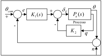
Overall delay is T = T_sens+T_c / 2+T_s; delay is modelled with an II order Padè approximation, that will be multiply SISO dynamic transfer function that we have considered on loop control definition.

Multi-loop logic scheme for longitudinal dynamics

Closed-loop behaviour, with four controllers discretized by Tusting method with step T=0.01, was analyzed with a non-linear simulation, within a Matlab/Simulink environment.

Controller summary

roll and pitch: ACAH, multi-loop
yaw and vertical speed: RCAH, single-loop